COMPSCI180_website
CS 180 Project 2: Fun with Filters and Frequencies
Part 1: Fun with Filters
In this part, we will build intuitions about 2D convolutions and filtering.
Part 1.1: Finite Difference Operator
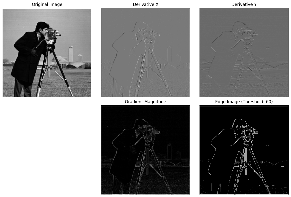
We will begin by using the humble finite difference as our filter in the x and y directions.
\[D_x = \begin{bmatrix}1 & -1\end{bmatrix}, D_y = \begin{bmatrix}1 \\-1\end{bmatrix}\]The gradient magnitude calculation involves the following theoretical steps:
-
Image Representation: The image is represented as a 2D array of pixel intensities.
-
Derivative Operators: Two derivative operators are defined:
-
Horizontal Derivative Operator (D_x): Detects changes in the horizontal direction. Vertical Derivative Operator (D_y): Detects changes in the vertical direction. Convolution: The image is convolved with the horizontal and vertical derivative operators to compute the derivatives in the x and y directions. This step highlights the intensity changes in the respective directions.
-
Gradient Magnitude Calculation: The gradient magnitude at each pixel is computed using the formula:
\[\text{gradient_magnitude} = \sqrt{\text{derivative_x}^2 + \text{derivative_y}^2}\]This combines the horizontal and vertical derivatives to give the overall edge strength at each pixel.
-
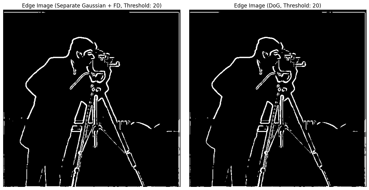
Edge Detection: A threshold is applied to the gradient magnitude to create a binary edge image, where pixels with gradient magnitudes above the threshold are considered edges.
The Finite Difference Operator estimates image gradients by computing horizontal and vertical derivatives, which reveal intensity changes, indicating edges. It uses simple kernels to calculate these derivatives through convolution, and the gradient magnitude is derived by combining both directions. However, this method is sensitive to noise, as it directly processes raw pixel values. Edges are detected by thresholding the gradient magnitudes, making it a straightforward but noise-prone approach for edge detection. After multiple adjustments to the threshold and implementations, I found that the best result was achieved with a threshold of 60.
Part 1.2: Derivative of Gaussian (DoG) Filter
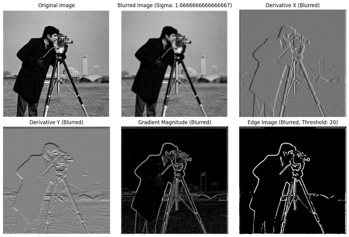
Firstly, create a blurred version of the original image by convolving with a gaussian and repeat the procedure in the previous part (using cv2.getGaussianKernel() to create a 1D gaussian and then taking an outer product with its transpose to get a 2D gaussian kernel).
The processed image clearly contains less noise and has more distinct edges.
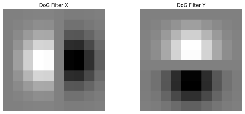
Then, do the same thing with a single convolution instead of two by creating a derivative of gaussian filters (DoG Filter)
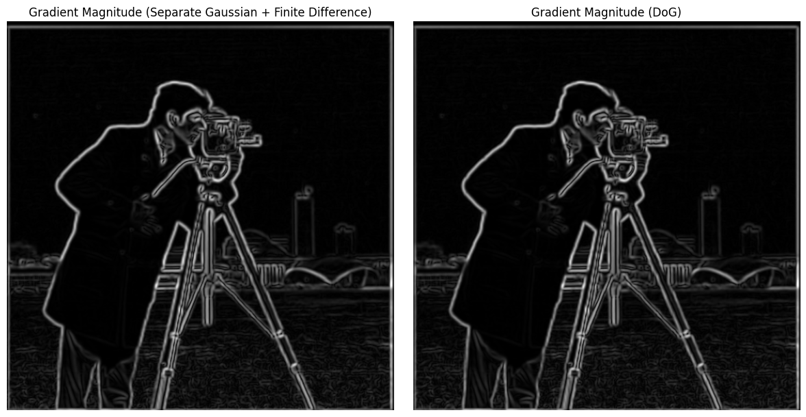
These two methods get the same result.
Part 2: Fun with Frequencies!
Part 2.1: Image “Sharpening”
The principle of sharpening an image by subtracting a Gaussian-blurred version from the original image is based on enhancing edges and fine details. In this process, the original image is first blurred using a Gaussian filter to reduce noise and smooth out the details. By subtracting this blurred image from the original, the high-frequency components (representing edges and details) are amplified. Steps:
-
Image Normalization: The input image is read and normalized to have pixel values in the range ([0, 1]).
-
Gaussian Blurring: A Gaussian blur is applied to the normalized image. This involves convolving the image with a Gaussian kernel, which smooths the image by averaging pixel values with their neighbors, weighted by a Gaussian function. Mathematically, the Gaussian function is given by:
\[G(x, y) = \frac{1}{2\pi\sigma^2} e^{-\frac{x^2 + y^2}{2\sigma^2}}\] -
High-Frequency Component Extraction: The high-frequency components of the image are extracted by subtracting the blurred image from the original image. This step isolates the details and edges in the image. If (I) is the original image and (B) is the blurred image, the high-frequency component (H) is:
\[H = I - B\] -
Sharpening: The high-frequency components are scaled by a factor ((\alpha)) and added back to the original image. This enhances the details and edges, making the image appear sharper. The sharpened image (S) is given by:
\[S = I + \alpha H = I + \alpha (I - B)\]
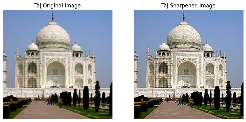

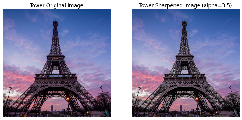
For a character image from GTA5, I first applied a blur and then sharpening, and found that the sharpening effect was significant.

GTA5

GTA5_blurred

GTA5_sharpened

GreatWall
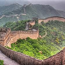
GreatWall_sharpened
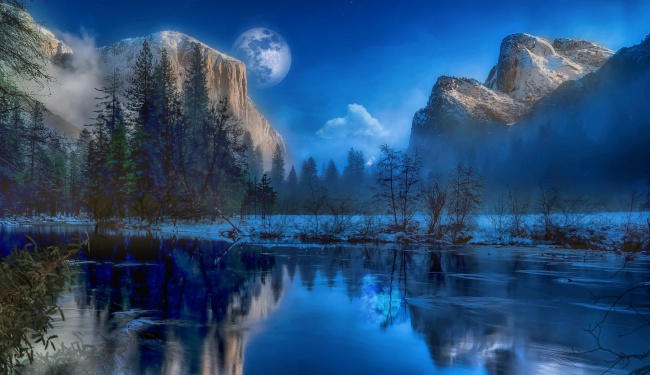
Sea

Sea_sharpened
Part 2.2: Hybrid Images
- Cropping and Resizing Images:
- Crop and resize two images to ensure they have the same dimensions. This step is essential for allowing effective blending in the later stages.
- Defining the Gaussian Function:
- Use the Gaussian function to model the filtering process. This function helps in determining how much each pixel contributes to the final image based on its distance from the center of the filter.
- Creating Filter Matrices:
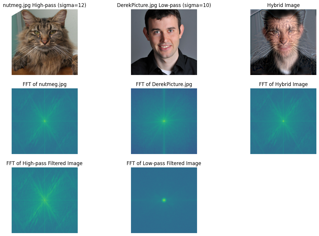
- Generate filter matrices for both low-pass and high-pass filtering. For low-pass filtering, I applied the Gaussian function directly to retain smooth features. In contrast, for high-pass filtering, I inverted the Gaussian to enhance the image’s edges and details.
- Applying Frequency Domain Filtering:
- Transforme the color channels of the images into the frequency domain using Fast Fourier Transform (FFT). This allows to apply the filter matrices effectively. After filtering, transform the images back to the spatial domain to retrieve the modified pixel values.
Bells & Whistles: Using color to enhance the effect, I found that both high-frequency and low-frequency images work best when their colors are preserved, so I chose to use color images for my work.
About bad results: My initial attempt resulted in an incorrect outcome because I did not consider that overlaying two images might cause pixel values to exceed the range of 255, leading to distortion in one of the RGB channels, manifesting as bizarre color artifacts. This was due to the lack of a normalization step.
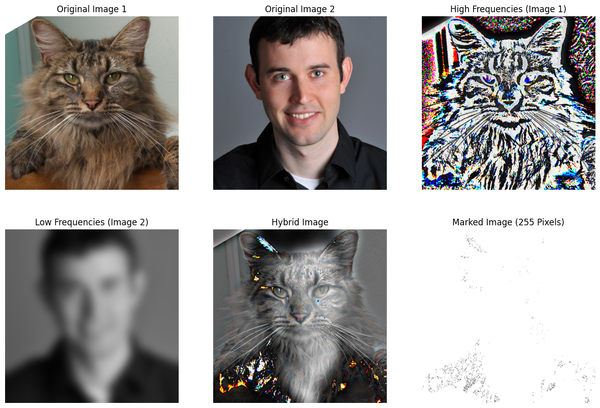
After fixing this bug, I got the perfect result:
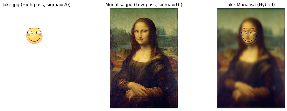
I like the game Elden Ring, so I decided to make a funny version of Melina.

There are also some funny ideas.

Multi-resolution Blending and the Oraple journey
Part 2.3: Gaussian and Laplacian Stacks
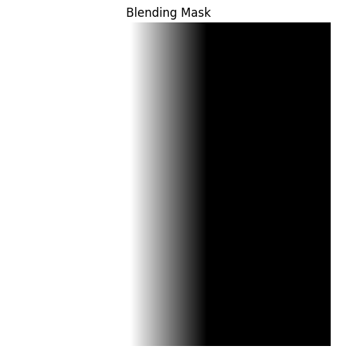
Implement a Gaussian and a Laplacian stack. The different between a stack and a pyramid is that in each level of the pyramid the image is downsampled, so that the result gets smaller and smaller. In a stack the images are never downsampled so the results are all the same dimension as the original image, and can all be saved in one 3D matrix (if the original image was a grayscale image).
Here is the process of creating stacks.


Apply the Gaussian and Laplacian stacks to the Oraple and recreate the outcomes of Figure 3.42 in Szelski (Ed 2) page 167.
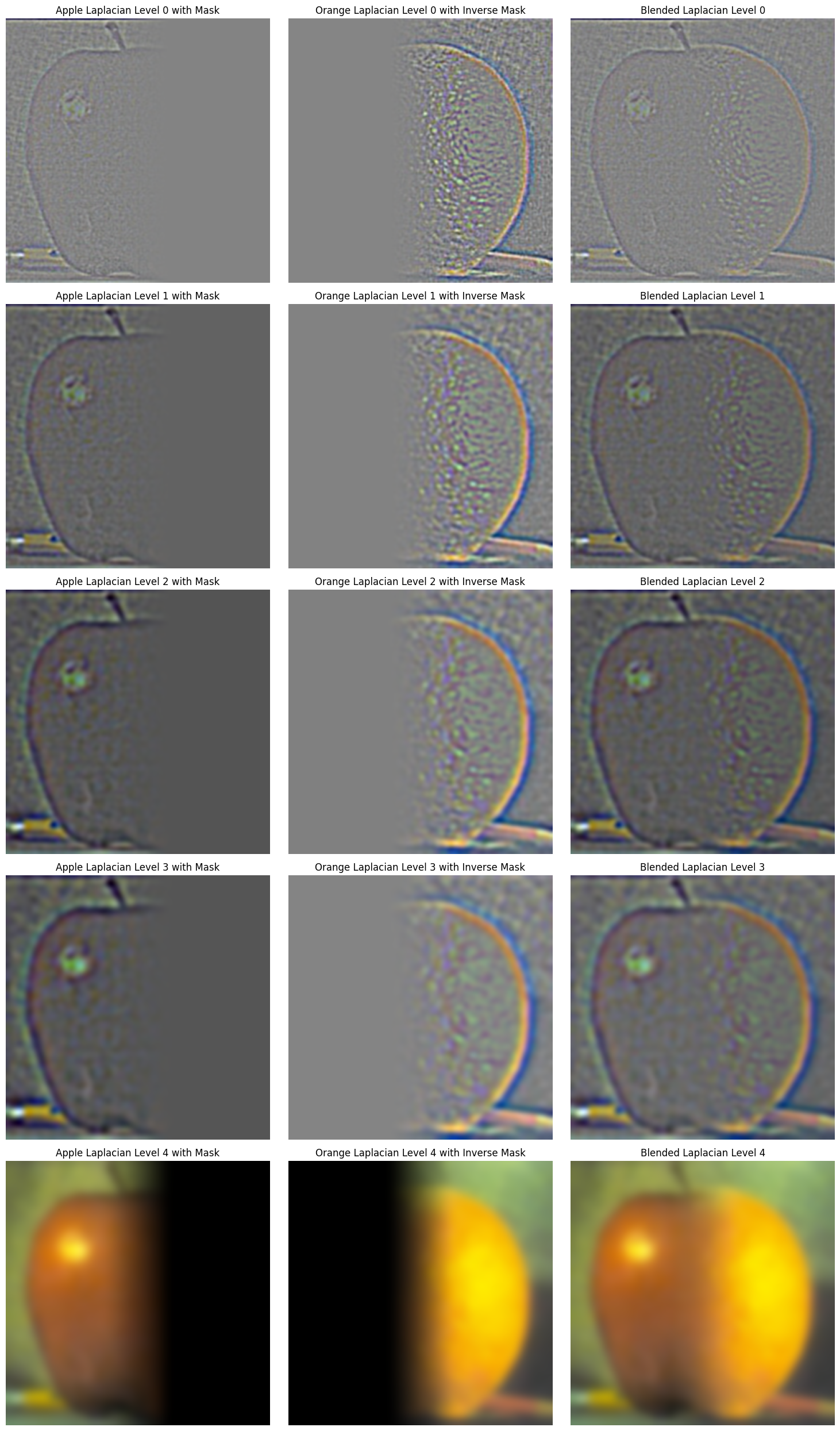

Part 2.4: Multiresolution Blending
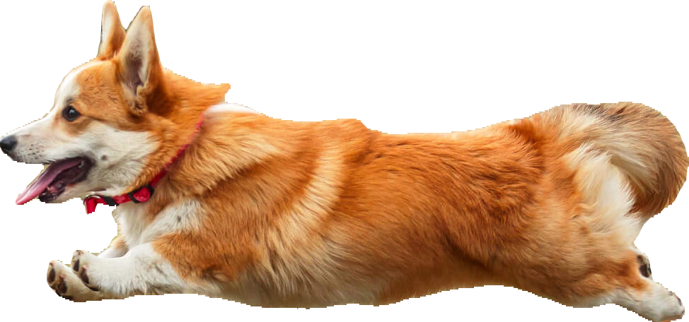
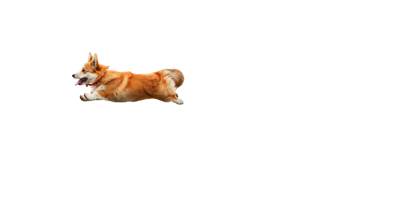
The masks are produced by Segment Anything (Research by Meta AI)
dog

plane
dog

mask
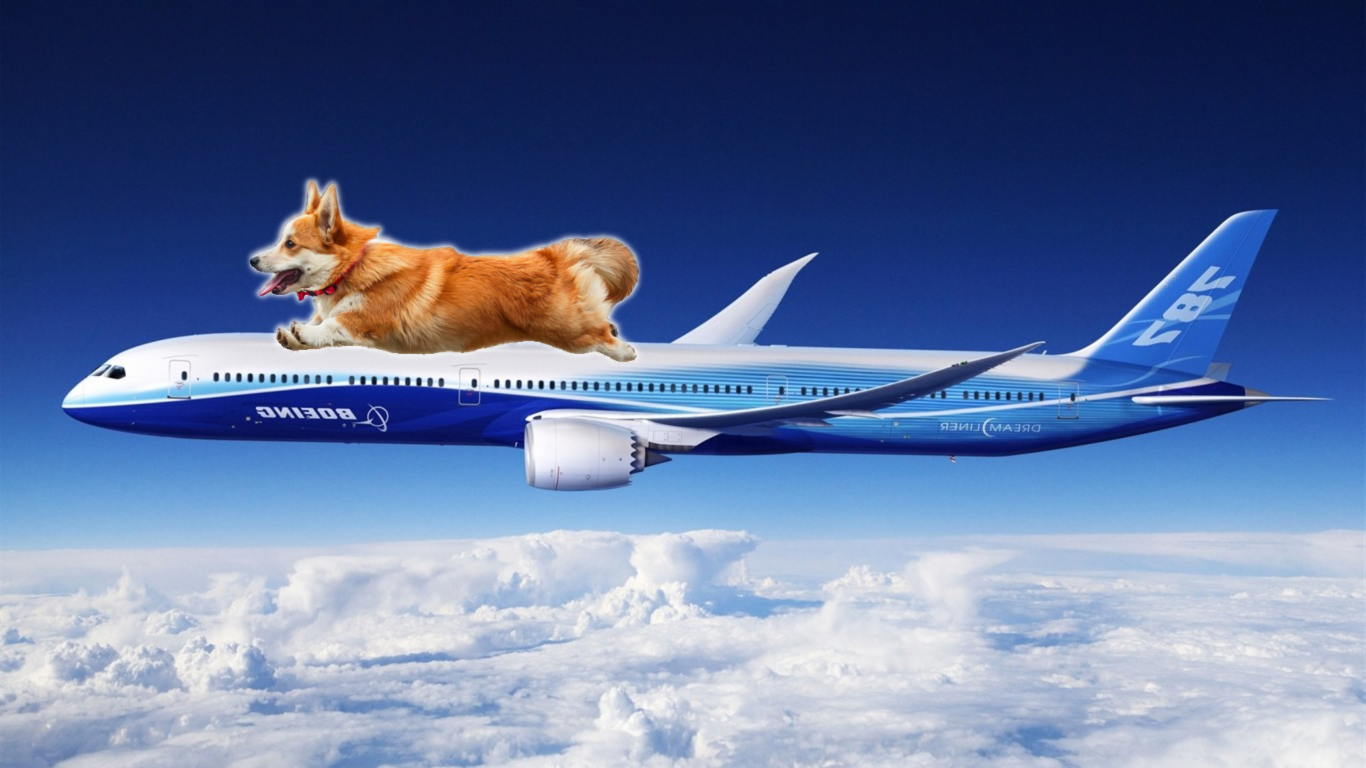
dog_plane

cat

cake
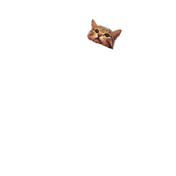
cat
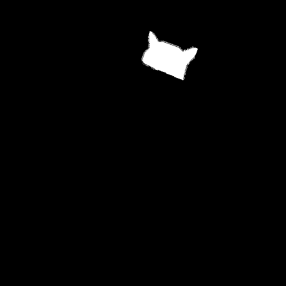
mask

cat_cake